综述
- 线性回归介绍
- 线性回归pmml 介绍
- 线性回归模型结构
- 如何手动写一个java类表述线性回归
很多时候,我们在看机器学习的算法的时候,看到的都是一些列的公式推导。那么这些公式推导出来的结果是什么?最后又是如何组织的?作为一个码农,更关心的是,这些公式最后又是如何变为代码的?
本系列将借助PMML这一工具,可以用来解析模型的结构,了解各种模型中都有那些元素?这些元素又是通过何种组合方式,计算公式得到最后的结果的?
本文针对偏工程人员,不涉及具体的模型优化求解问题,我们关注的是模型实质的结构,以及根据这些信息,如何实现跨平台的使用模型。至于模型的求解过程,前人已经总结完备,不过多赘述,在文中会给出地址,如有兴趣,可以自行查阅推导。
先从简单的线性回归开始
什么是线性回归
定义:1
在统计学中,线性回归(Linear Regression)是利用称为线性回归方程的最小平方函数对一个或多个自变量和因变量之间关系进行建模的一种回归分析。这种函数是一个或多个称为回归系数的模型参数的线性组合。只有一个自变量的情况称为简单回归,大于一个自变量情况的叫做多元回归。
线性回归是数据挖掘中的基础算法之一,从某种意义上来说,在学习函数的时候已经开始接触线性回归了,只不过那时候并没有涉及到误差项。线性回归的思想其实就是解一组方程,得到回归函数,不过在出现误差项之后,方程的解法就存在了改变,一般使用最小二乘法进行计算。
解决问题流程
Step1. 选择一个模型函数h
Step2. 为h找到适应数据的最优解,即找出最优解下的h的参数。
函数模型
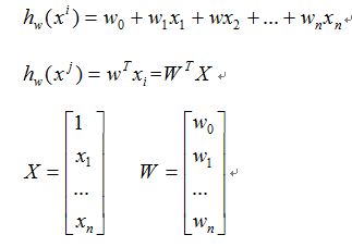
其中h()是一个线性函数,所有的自变量构成一个一维向量X,所有参数构成一个一维向量W,就可以将第一行的公式改写为第二行的形式。
假设存在训练数据集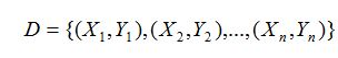
为了方便,可以改写为矩阵的形式
其中x可以看成特征,theater看成是权重。我们的目标就是找出所有的权重,进而出现新的x值时,可以对函数的输出进行估计。那我们如何求得使函数输出最接近样本的值呢?函数输出最接近样本值就意味着二者之差尽可能的小。我们假设输入的特征为,对应的样本值为,我们用模型估计出的值为,估计值与真实值之间的误差表示为
成为损失函数,损失函数的自变量为,所以我们需要找到最小时的取值。
在机器学习中我们采用梯度下降算法求解该方程,
一般的求解方法有梯度下降法,牛顿法,共轭梯度法,启发式优化方法等,在这篇博文中介绍的比较详细。再次不多赘述。
OK,通过求解损失函数最小化,我们会得到一组参数,这就是线性回归的解,根据这个解,就有了我们的模型。
操作实例
sklearn 实现线性回归
1 | from sklearn2pmml import PMMLPipeline |
以上是希望拟合y=0.5 x1 + 0.5 x2。
测试下1
pipeline.predict([[1.0,2.0]])
结果为:1.5 符合预期
将其导出为pmml1
sklearn2pmml(pipeline,"linearregression.pmml",with_repr = True)
线性回归的PMML及结构
上一节中的模型,导出PMML文件的主要部分如下:1
2
3
4
5
6
7
8
9
10
11
12
13
14
15
16<DataDictionary>
<DataField name="y" optype="continuous" dataType="double"/>
<DataField name="x1" optype="continuous" dataType="double"/>
<DataField name="x2" optype="continuous" dataType="double"/>
</DataDictionary>
<RegressionModel functionName="regression">
<MiningSchema>
<MiningField name="y" usageType="target"/>
<MiningField name="x1"/>
<MiningField name="x2"/>
</MiningSchema>
<RegressionTable intercept="2.220446049250313E-16">
<NumericPredictor name="x1" coefficient="0.4999999999999999"/>
<NumericPredictor name="x2" coefficient="0.49999999999999983"/>
</RegressionTable>
</RegressionModel>
模型一共两个输入 x1 x2,一个目标输出y
x1,x2 对应的参数分别为 0.4999999999999999 和 0.49999999999999983 (注意,这里不是0.5,是因为拟合的误差原因)整个的截距是2.220446049250313E-16
只要有了这几个参数,你就有了训练好的模型。针对任意的输入的x1,x2,你都能直接输入一个拟合好的y,掉包 不存在的。
用Scala实现线性回归的预测
这里,参考了Spark MLlib中的源码,简单写了几个类,主要用于说明线性回归的结构,以及预测的逻辑。没有涉及到模型的训练。
从上一节中,可以看出线性回归模型中,其实就两个参数,1个权重向量,1个截距。
1 | class LinerRegressionModel( |
定义线性回归模型,预测结果是输入向量和权重向量点积加上截距。
权重向量就是上边每个入参对应的参数。
测试类如下:1
2
3
4
5
6
7
8def testLinerRegression(): Unit ={
val weight = Array(0.4999999999999999, 0.49999999999999983)
val intercept = 2.220446049250313E-16
val model = new LinerRegressionModel(weight,intercept)
val x = Array(1.0, 2.0)
val y = model.predict(x)
println(f"The Result Of Model is ${y}")
}
预测(1.0, 2.0)结果为:1
The Result Of Model is 1.4999999999999998
四舍五入和python结果一致。
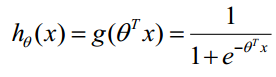
逻辑回归
根据上文的叙述,线性回归的模型是求出输出特征向量Y和输入样本矩阵X之间的线性关系系数theater,使其满足Y=theater X,如果的Y是连续的,所以是回归模型。如果我们想要Y是离散的话,怎么办呢?一个可以想到的办法是,我们对于这个Y再做一次函数转换,变为g(Y)。如果我们令g(Y)的值在某个实数区间的时候是类别A,在另一个实数区间的时候是类别B,就可以得到一个分类模型。
在逻辑回归中,这个函数就是sigmoid函数
下图展示了将分布函数变形的过程。

具体的求解过程,可以参见这篇文章的叙述,本文不做赘述http://www.aboutyun.com/thread-10650-1-1.html
二元逻辑回归
如果结果的类别只有两种,那么就是一个二元分类模型了。
二元逻辑回归的预测值由下式求得
因此,逻辑回归分类器的解就是一组权值向量,和线性回归是一致的。
二元逻辑回归python实现
使用自带的iris数据集进行操作,iris中包含3个分类,为了体现二分类的特性,删除了一个分类。1
2
3
4
5
6
7
8
9
10
11
12
13
14
15
16
17
18
19
20from sklearn2pmml import PMMLPipeline
from sklearn2pmml import sklearn2pmml
from sklearn.datasets import load_iris
from sklearn.linear_model import LogisticRegression
from sklearn.model_selection import train_test_split
import pandas as pd
import numpy as np
lr = LogisticRegression()
# 导入数据,为了后续方便,将三类中的一类去除,使之变为二分类问题。
iris = load_iris()
df = pd.DataFrame(iris.data)
df["class"] = iris.target
df.columns=['V0','V1','V2','V3','class']
df = df[df['class'] < 2]
df.describe()
X_train, X_test, y_train, y_test = train_test_split(df[df.columns.difference(['class'])], df['class'], test_size=0.5, random_state=42)
pipeline = PMMLPipeline([("classifier", lr)])
pipeline.fit(X_train,y_train)
然后将训练好的模型导出为PMML1
2from sklearn2pmml import sklearn2pmml
sklearn2pmml(pipeline, "LRbin.pmml", with_repr = True)
二元逻辑回归PMML分析
上一节代码生成的PMML中的主要部分如下:1
2
3
4
5
6
7
8
9
10
11
12
13
14
15
16
17
18
19
20
21
22
23
24
25
26
27
28
29
30<DataDictionary>
<DataField name="class" optype="categorical" dataType="integer">
<Value value="0"/>
<Value value="1"/>
</DataField>
<DataField name="V0" optype="continuous" dataType="double"/>
<DataField name="V1" optype="continuous" dataType="double"/>
<DataField name="V2" optype="continuous" dataType="double"/>
<DataField name="V3" optype="continuous" dataType="double"/>
</DataDictionary>
<RegressionModel functionName="classification" normalizationMethod="logit">
<MiningSchema>
<MiningField name="class" usageType="target"/>
<MiningField name="V0"/>
<MiningField name="V1"/>
<MiningField name="V2"/>
<MiningField name="V3"/>
</MiningSchema>
<Output>
<OutputField name="probability(0)" optype="continuous" dataType="double" feature="probability" value="0"/>
<OutputField name="probability(1)" optype="continuous" dataType="double" feature="probability" value="1"/>
</Output>
<RegressionTable intercept="-0.24391923532173168" targetCategory="1">
<NumericPredictor name="V0" coefficient="-0.31738779611631857"/>
<NumericPredictor name="V1" coefficient="-1.2346299390640323"/>
<NumericPredictor name="V2" coefficient="1.920449906205768"/>
<NumericPredictor name="V3" coefficient="0.8753093733469249"/>
</RegressionTable>
<RegressionTable intercept="0.0" targetCategory="0"/>
</RegressionModel>
一共四个入参,V0,V1,V2,V4 都为double类型。目标输出为0,1分类。
模型是一个classification,标准化使用的是logit函数,也就是sigmod函数。
权重矩阵为(-0.31738779611631857,-1.2346299390640323,1.920449906205768,0.8753093733469249),截距为-0.24391923532173168。
这里需要注意,二分类只需要一个RegressionTable就能满足分类的需求,后续的多分类会涉及到多个RegressionTable。
这里就能发现,二分类的LR,其实就是对输入求了一次线性回归的值,然后对这个值再求其sigmod解。因而,有了权重矩阵和截距,我们就能求出逻辑回归的预测值。
scala简单实现
定义一个用于二元逻辑回归计算预测概率值的类。1
2
3
4
5
6
7
8
9
10
11
12
13
14
15
16
17class LRBinModel(
val weights: Array[Double],
val intercept: Double) {
def predict(testData:Array[Double]): Double ={
predictPoint(testData,weights,intercept)
}
def predictPoint(
dataMatrix: Array[Double],
weightMatrix: Array[Double],
intercept: Double): Double = {
val margin = DenseVector(dataMatrix).dot(DenseVector(weightMatrix)) + intercept
val score = 1.0 / (1.0 + math.exp(-margin))
score
}
}
取测试集的第一条记录,进行测试1
2
3
4
5X_t=X_test.head(1)
print(X_t)
y_t=y_test.head(1)
print(y_t)
pipeline.predict_proba(X_t)
可以看到,第一条记录的数据为1
6.0 2.7 5.1 1.6
实际类别为1
预测结果为1
array([[ 0.00329174, 0.99670826]])
意为属于类别0的概率为0.0032917,属于类别1的概率为0.99670826,两者的和正好为1。故而,求出为类别1的概率之后,用1减去该值就为类别0的概率。
编写一个简单的测试方法,测试改组数据1
2
3
4
5
6
7
8
9def testLRbin(): Unit ={
val weight = Array(-0.31738779611631857,-1.2346299390640323,1.920449906205768,0.8753093733469249)
val intercept = -0.24391923532173168
val model = new LRBinModel(weight, intercept)
val x = Array(6.0, 2.7, 5.1, 1.6)
val y = model.predict(x)
println(f"The Probability Of Class 1 is ${y}")
}
结果为:1
The Probability Of Class 1 is 0.9967082628300301
属于类别1的概率为0.9967082628300301 和python 的预测结果基本一致。
然后就可以根据设定的阈值,判别属于哪一类了。
模型中的调优参数
对于逻辑回归模型,会有一些参数需要调节,比如C,max_iter,penalty等,这几个值在模型求解的过程中生效,在已经求解的模型中,并无体现。
多元逻辑回归分析
多元逻辑回归,和二元类似,分别计算属于每个类别的概率,选取其中的最大值作为预测值。具体叙述参见
多元逻辑回归python实现
我们还是使用iris数据集进行示例,这次不用删除类别了。1
2
3
4
5
6
7
8
9
10
11from sklearn2pmml import PMMLPipeline
from sklearn.datasets import load_iris
from sklearn.linear_model import LogisticRegression
iris = load_iris()
clf = LogisticRegression()
pipeline = PMMLPipeline([("classifier", clf)])
pipeline.fit(iris.data, iris.target)
# 导出为PMML
from sklearn2pmml import sklearn2pmml
sklearn2pmml(pipeline, "LR.pmml", with_repr = True)
多元逻辑回归PMML分析
1 | <DataDictionary> |
基本上和二元逻辑回归类似,只是RegressionTable 有三个,这是因为一共有三个类别,需要三组权重矩阵和截距,分别计算属于当前类别的概率值,因而对于多元逻辑回归而言,有多少元,输出的概率值就有多少个。
然后再针对所有输出的概率,求和,然后计算每个概率和求和概率的比值。这是为了保证形式上的统一。
Scala实现
1 | class LRMultiModel( |
对于python训练的模型,选取head(1)进行测试1
2
3
4
5X_t=X_test.head(1)
print(X_t)
y_t=y_test.head(1)
print(y_t)
pipeline.predict_proba(X_t)
结果如下:1
[[ 0.00122453 0.39920192 0.59957355]]
编写测试方法测试1
2
3
4
5
6
7
8
9
10
11
12
13
14
15
16
17
18
19
20
21
22
23def testLRMul(): Unit ={
val weight = Array(
Array(0.4149883282957013,1.4612973885622267,-2.2621411772020728,-1.02909509924489),
Array(0.41663968559520786,-1.6008331852575897,0.5776576286775582,-1.3855384286634223),
Array(-1.7075251538239047,-1.5342683399889876,2.4709716807720206,2.5553821129820884)
)
val intercept = Array(0.26560616797551695, 1.0854237423889572, -1.2147145780786366)
val model = new LRMultiModel(weight, intercept)
val x = Array(6.0, 2.7, 5.1, 1.6)
val y = model.predict(x)
var mclass = 0
var max = 0.0
for (i <- 0 until y.size){
println(f"The Probability Of Class ${i} is ${y(i)}")
if (y(i) > max){
max = y(i)
mclass = i
}
}
println(s"The Class May Be ${mclass}")
}
结果如下:1
2
3
4The Probability Of Class 0 is 0.0012245308619260621
The Probability Of Class 1 is 0.39920191920408243
The Probability Of Class 2 is 0.5995735499339914
The Class May Be 2
两者完全一致。
总结
本文借助了PMML,解析了简单线性回归和逻辑回归的结构。介绍了这两种模型是如何实现预测的。其实所有看起来,或者听起来“高大上”的模型,在码农的眼里,最终的呈现都是一系列的“参数”而已。
通过不同的方式将这些参数组合起来,便可实现一些神奇的功能。
REF
https://blog.csdn.net/fleurdalis/article/details/54931721
李航 统计学习方法